plot_radial

A function for producing radial IVW and MR-Egger plots either individually or simultaneously. The function allows for a variety of aesthetic and scaling options, utilising the output from the IVW_radial and egger_radial functions.

Usage

plot_radial(r_object, radial_scale, show_outliers, scale_match)

Arguments

r_object

An object of class "IVW" or "egger". For visualising both estimates simultaneously, both objects should be included as a vector c(A,B), where A and B denote the "IVW" and "egger" objects respectively.

radial_scale

Indicates whether to produce a plot including a full radial scale (TRUE), or a scatterplot showing only the effect estimates (FALSE).

show_outliers

Indicates whether display only the set of variants identified as outliers (TRUE) or the complete set of variants (FALSE). Note that when (show_outliers=TRUE), non-outlying variants further from the origin than the furthest outlier will cause an error message that one or more points have been omitted. These are non-outlying variants beyond the scale. If no outliers are present, a plot will be produced using the full set of variants, with an accompanying message indicating the absence of outliers.

scale_match

Indicates whether x and y axes should have the same range(TRUE), or different ranges (FALSE) This improves the interpretation of the radial scale, and is set to FALSE when the radial scale is omitted from the plot.

Value

A ggplot object containing a radial plot of either the IVW, MR-Egger, or both estimates simultaneously.

References

Bowden, J., et al., Improving the visualization, interpretation and analysis of two-sample summary data Mendelian randomization via the Radial plot and Radial regression. International Journal of Epidemiology, 2018. 47(4): p. 1264-1278.

Author

Wes Spiller; Jack Bowden; Tom Palmer.

Examples

ldl.dat <- data_radial[data_radial[,10]<5e-8,]
ldl.fdat <- format_radial(ldl.dat[,6], ldl.dat[,9],
                          ldl.dat[,15], ldl.dat[,21], ldl.dat[,1])
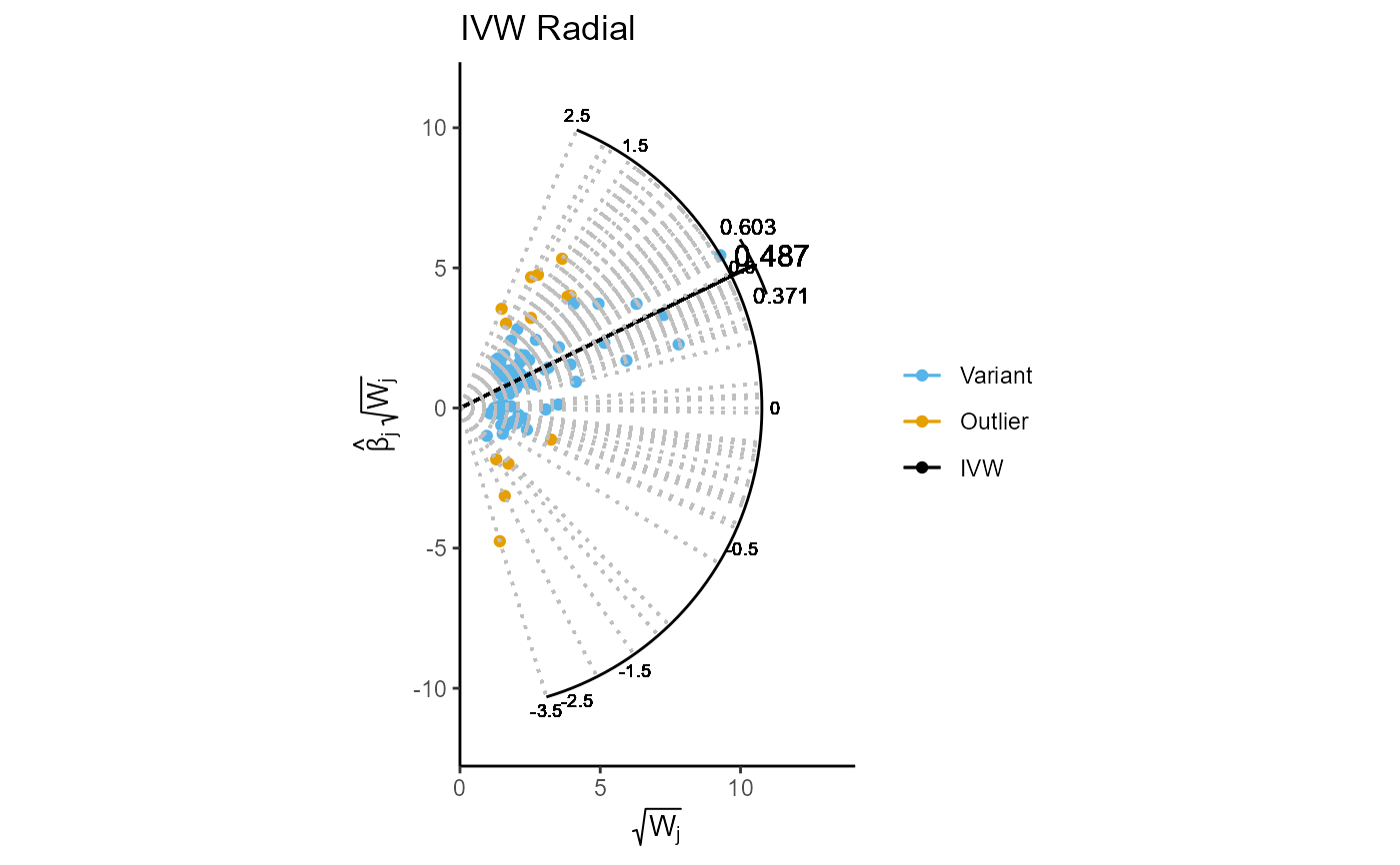
ivw.object <- ivw_radial(ldl.fdat, 0.05, 1, 0.0001, TRUE)
#> 
#> Radial IVW
#> 
#>               Estimate  Std.Error   t value     Pr(>|t|)
#> Effect (1st) 0.4874900 0.05830409  8.361163 6.210273e-17
#> Iterative    0.4873205 0.05827885  8.361874 6.172955e-17
#> Exact (FE)   0.4958973 0.03804168 13.035630 7.673061e-39
#> Exact (RE)   0.4910400 0.05387806  9.113916 4.729550e-14
#> 
#> 
#> Residual standard error: 1.544 on 81 degrees of freedom
#> 
#> F-statistic: 69.91 on 1 and 81 DF, p-value: 1.46e-12
#> Q-Statistic for heterogeneity: 193.0843 on 81 DF , p-value: 3.827332e-11
#> 
#>  Outliers detected 
#> Number of iterations = 3
plot_radial(ivw.object)

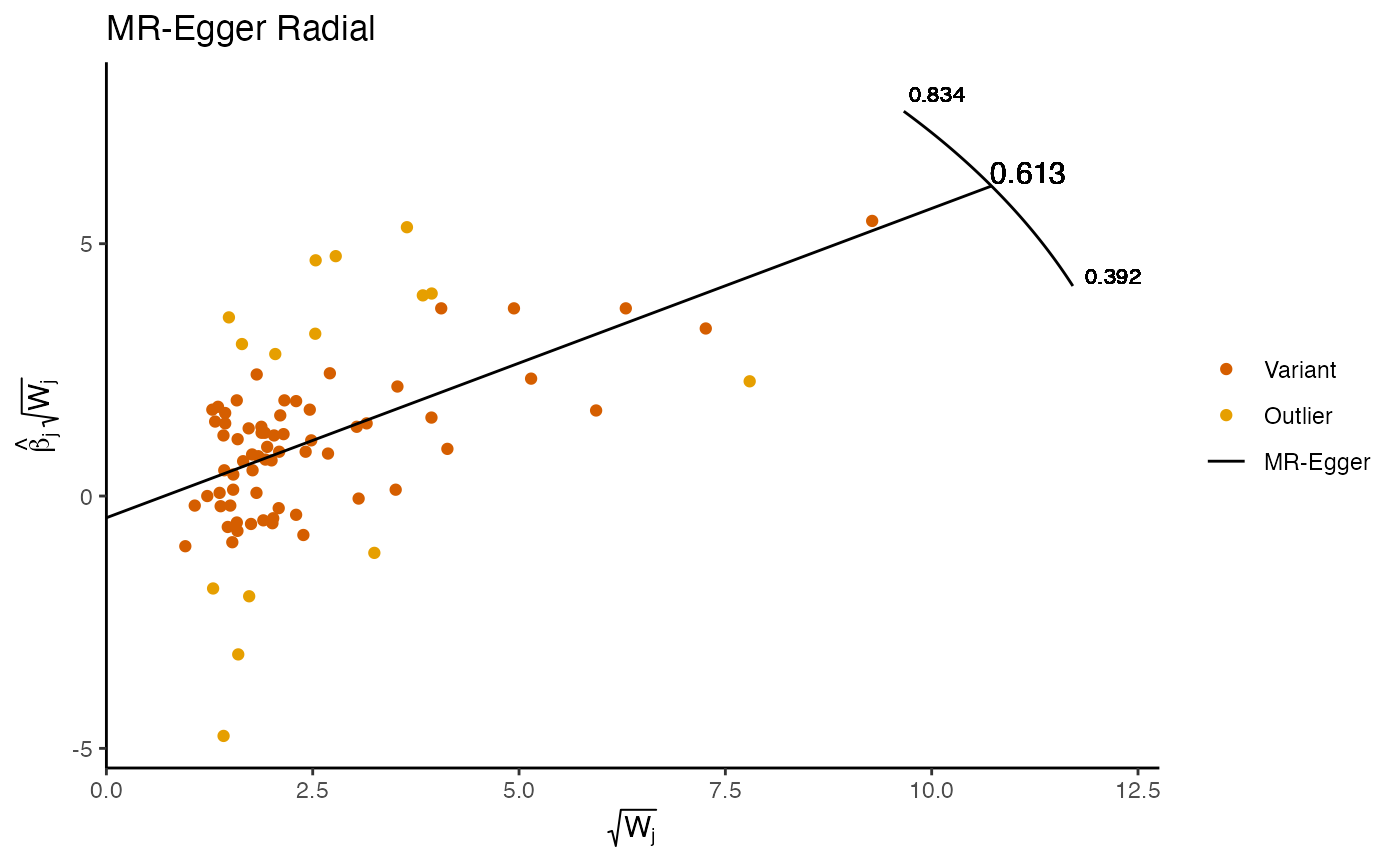
egg.object <- egger_radial(ldl.fdat, 0.05, 1, TRUE)
#> 
#> Radial MR-Egger
#> 
#>               Estimate Std. Error   t value     Pr(>|t|)
#> (Intercept) -0.4303552  0.3244151 -1.326557 1.884296e-01
#> Wj           0.6129126  0.1109369  5.524877 3.988423e-07
#> 
#> Residual standard error: 1.537 on 80 degrees of freedom
#> 
#> F-statistic: 30.52 on 1 and 80 DF, p-value: 3.99e-07
#> Q-Statistic for heterogeneity: 188.9285 on 80 DF , p-value: 8.445607e-11
#> 
#>  Outliers detected 
#> 
plot_radial(egg.object)